Dog Breed Classification
An end-to-end computer vision pipeline in PyTorch built to tell Collies apart from Golden Retrievers. I implemented a CNN, a transfer learning system, and a Vision Transformer from first principles, then used what those experiments taught me to design a custom architecture of my own.
Working title: "Paco's Puppy Problem"
Four ways to teach a model to see a dog.
Every image in this dataset is a 64x64 RGB photo of a dog, one of ten breeds, split into training, validation, testing, and a held-out challenge partition. The target task is binary: tell Collies apart from Golden Retrievers. A related source task uses the other eight breeds, Samoyed, Miniature Poodle, Saint Bernard, Great Dane, Dalmatian, Chihuahua, Siberian Husky, and Yorkshire Terrier, to test whether visual features learned on one classification problem transfer to another.
Rather than building one classifier, this project moved through four stages: a convolutional network built from scratch, a transfer learning system that reused those learned features, a Vision Transformer implemented layer by layer, and finally a custom CNN designed from what the earlier experiments revealed. Each stage is its own small investigation into how these architectures learn, overfit, and generalize.
Learning to see, before learning to classify.
Before any model sees an image, every channel gets standardized. I implemented an ImageStandardizer that fits a per-channel mean and standard deviation using only the training partition, then applies that same transform to validation, test, and challenge data. Fitting on training data alone matters: if validation or test statistics leaked into the transform, the model would be indirectly evaluated on information it was never supposed to see.
def fit(self, X: npt.NDArray) -> None:
X = X.astype(np.float64)
self.image_mean = np.mean(X, axis=(0, 1, 2))
self.image_std = np.std(X, axis=(0, 1, 2))
def transform(self, X: npt.NDArray) -> npt.NDArray:
eps = 1e-8
return (X - self.image_mean) / (self.image_std + eps)
Learned statistics
The training partition's per-channel mean came out to [125.55, 118.79, 94.77] and standard deviation to [64.41, 61.38, 64.25] for red, green, and blue. Those six numbers are the only thing every downstream model ever learns about the raw pixel distribution.
Why this preserves signal
Standardized images look slightly softer and less saturated, but every shape, edge, and texture a classifier needs is still fully intact. Normalization changes the input scale, not the content.
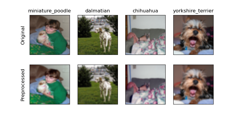
Original images (top) versus their standardized versions (bottom). The transform changes pixel scale without losing visual structure.
A convolutional network, built from scratch.
The baseline model, which I'll call the Target CNN, is three convolutional blocks feeding a single fully connected layer. Each convolution uses a 5x5 kernel with stride 2 and same padding, followed by ReLU, with max pooling after the first two. I implemented the layer definitions, Kaiming-style weight initialization, and the forward pass directly in PyTorch, along with the full training loop: zero gradients, forward pass, cross-entropy loss, backward pass, optimizer step.
x = F.relu(self.conv1(x))
x = self.pool(x)
x = F.relu(self.conv2(x))
x = self.pool(x)
x = F.relu(self.conv3(x))
x = x.view(x.size(0), -1)
return self.fc_1(x)
Working through the parameter count by hand before writing any code, 1,216 for the first convolution, 25,664 for the second, 12,808 for the third, and 66 for the fully connected layer, gave a total of 39,754 learnable parameters, which matched the program's output exactly once the model was implemented.
More patience, more capacity, not automatically better.
Two early experiments shaped how I thought about the rest of the project. The first compared early-stopping patience values of 5 and 10. The second widened the final convolutional layer from 8 filters to 64. Neither change was free, and both taught the same lesson from a different angle: more of something is not the same as better.
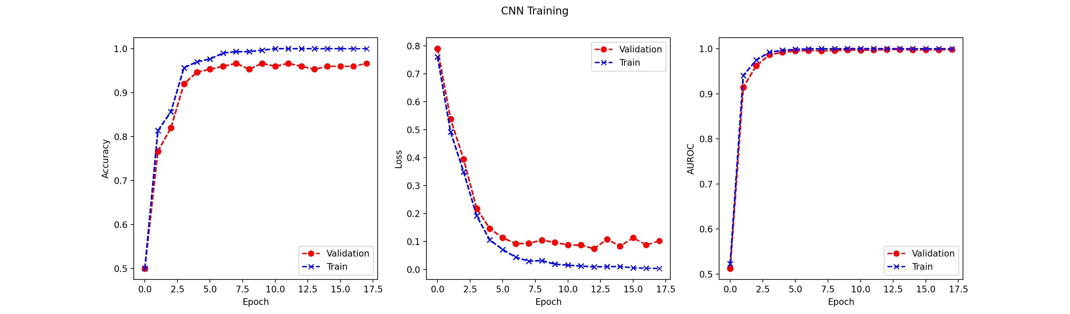
With patience 5, training stopped at epoch 17. The lowest validation loss had already occurred back at epoch 12, meaning the last five epochs were mostly polishing training loss toward zero rather than improving generalization.
Patience 5 worked slightly better. Patience 10 trained longer but the validation loss plateaued in the same place, around epoch 12, while training loss kept dropping, a sign the extra epochs were feeding overfitting rather than real improvement. Increased patience would matter more on a noisier or slower-converging training curve; here it just meant more time spent memorizing.
| Final conv layer | Best epoch | Training AUROC | Validation AUROC |
|---|---|---|---|
| 8 filters | 12 | 1.0000 | 0.9980 |
| 64 filters | 6 | 0.9999 | 0.9952 |
Widening the last convolutional layer from 8 to 64 filters raised the fully connected input from 32 to 256 features. The wider model converged faster, reaching its best checkpoint at epoch 6 instead of 12, but its validation AUROC came in slightly lower. With a dataset this size, the extra capacity had more room to fit training-specific noise than to learn anything generalizable.
A validation AUROC of 0.998, and a test AUROC of 0.763.
Trained with a patience of 5 and 8 filters in the last convolutional layer, the baseline CNN's full scorecard told two different stories depending on which number you looked at.
| Training | Validation | Testing | |
|---|---|---|---|
| Accuracy | 1.0000 | 0.9600 | 0.6000 |
| AUROC | 1.0000 | 0.9980 | 0.7632 |
The train-validation gap alone is small and unremarkable. It's the validation-test gap that's the real story: a model that looks nearly perfect on validation dropped to 0.763 AUROC on genuinely unseen data. Inspecting the images themselves offered a hypothesis for why.
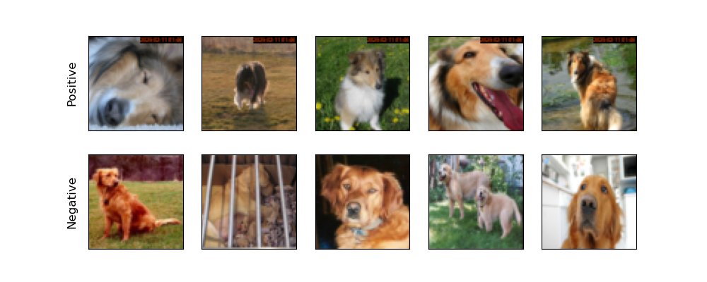
Positive-labeled Collies (top) versus negative-labeled Golden Retrievers (bottom)
Beyond the obvious breed traits, coat texture, ear shape, muzzle length, the two sets of images also differ in background and lighting. It's plausible the model picked up on some of that context alongside genuine breed features. That would explain the pattern exactly: strong performance wherever validation images resemble training images in ways that have nothing to do with the dog, and a real drop wherever the test set's conditions differ.
Strong validation performance can still be misleading when the validation data resembles the training data more closely than the true deployment distribution does.
Reusing what a network already learned to see.
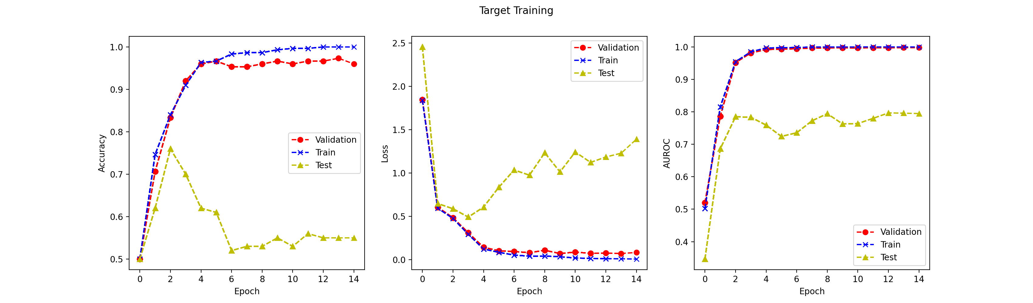
If the target CNN was struggling with limited, possibly context-biased data, one fix was to give it a better starting point. I trained a second CNN, the Source model, on the other eight breeds, then transferred its learned convolutional weights to the Collie-versus-Golden-Retriever task, freezing anywhere from zero to all three convolutional layers before fine-tuning.
The Source model reached its lowest validation loss, 1.7792, at epoch 8. After that, training accuracy kept climbing while validation performance flattened, which is exactly why checkpointing on validation loss rather than the final epoch matters.
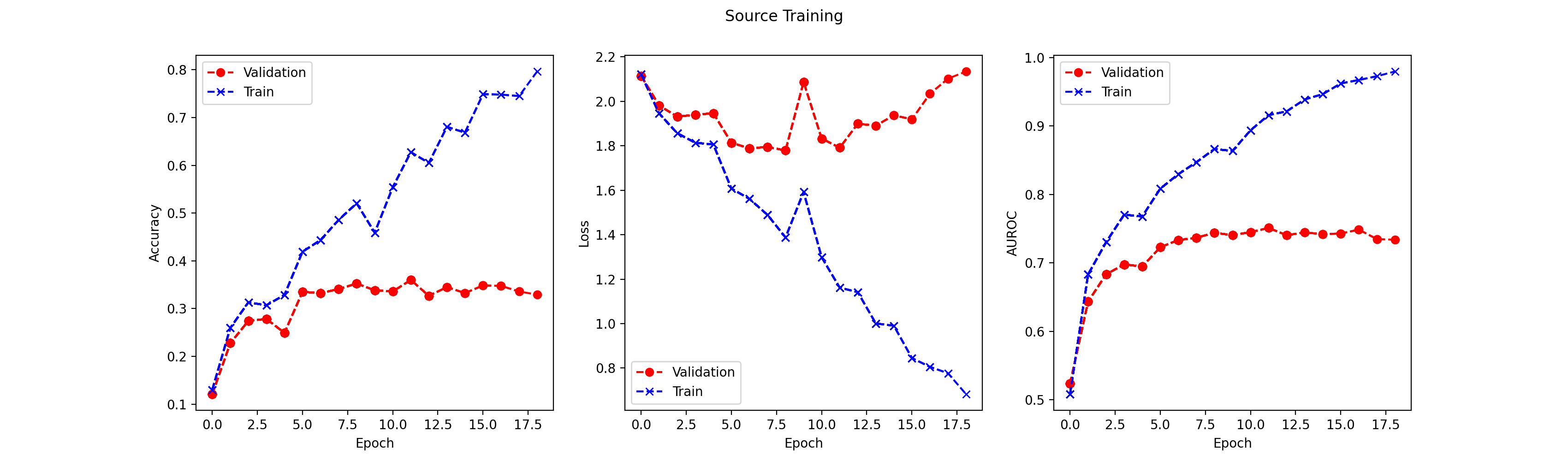
Source model training on the 8-breed classification task, patience 10
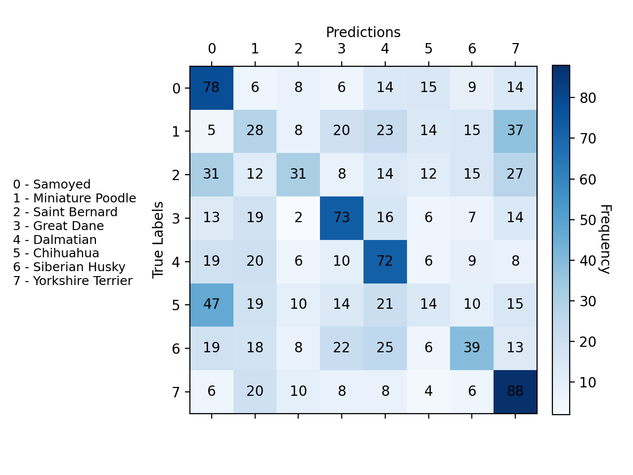
Confusion matrix on the validation set. Yorkshire Terrier and Samoyed were classified most reliably; Chihuahua and Saint Bernard were confused most often, likely due to visual overlap with other breeds in the set.
Freezing layers, one at a time
This is the most counterintuitive result in the project. Select a freezing configuration below to see its training curve.
| Strategy | Train | Validation | Test |
|---|---|---|---|
| Freeze all conv layers (fine-tune FC only) | 0.9018 | 0.9332 | 0.8264 |
| Freeze first 2 conv layers | 1.0000 | 0.9918 | 0.7512 |
| Freeze first conv layer | 1.0000 | 0.9979 | 0.7680 |
| Freeze no layers | 0.9999 | 0.9973 | 0.7628 |
| No pretraining or transfer learning | 1.0000 | 0.9980 | 0.7632 |
Freezing all three convolutional layers produced the lowest validation AUROC of any transfer configuration, 0.9332, yet the highest test AUROC by a wide margin, 0.8264. Every other configuration, including full fine-tuning, scored better on validation and worse on the held-out test set. Frozen, pretrained features acted like a strong regularizer: with every convolutional weight fixed, the model could only learn a linear combination of general dog features in its final layer, which left it with nowhere to overfit to validation-specific shortcuts. Letting every layer adapt gave the model the freedom to re-learn those same shortcuts, right back to where the original CNN started.
Reusing fixed visual features generalized better than fully fine-tuning the network, even though full fine-tuning looked stronger on the validation set.
A newer architecture, not a better one here.
Vision Transformers apply the attention mechanism from language models directly to images, splitting a picture into patches and treating each one as a token. I implemented the core pieces myself: patch-to-token projection, a learnable classification token, scaled dot-product attention, multi-head attention, and the transformer encoder blocks that stack on top.
scores = (q @ k.T) / self.scale_factor
weights = self.softmax(scores)
attention = weights @ v
Trained with 2 attention heads and 2 transformer blocks at an embedding dimension of 16, the model came out to roughly 7,394 learnable parameters, about a fifth the size of the baseline CNN.
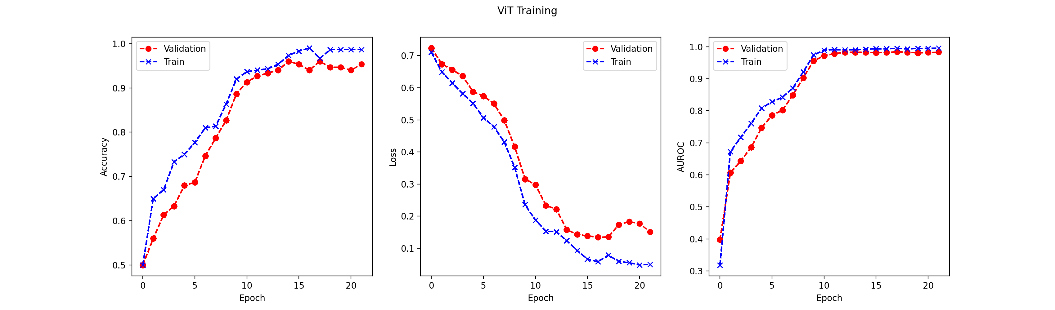
ViT training on the target task, patience 5. Lowest validation loss of 0.1431 at epoch 14.
| Model | Parameters | Validation AUROC | Test AUROC |
|---|---|---|---|
| Baseline CNN | 39,754 | 0.9980 | 0.7632 |
| Vision Transformer | 7,394 | 0.9826 | 0.6888 |
Despite being far smaller, the ViT didn't outperform the CNN, and actually generalized worse to the test set. CNNs carry useful spatial assumptions baked directly into their architecture: local receptive fields, shared filters, translation-aware feature extraction. Transformers have to learn spatial structure from data instead of assuming it, which usually takes a lot more data than 8,867 images to pay off. Architectural novelty didn't guarantee a better result here; the CNN's built-in assumptions were simply a better fit for a small image dataset.
Turning three experiments into one architecture.
For the final challenge, I had full control: architecture, initialization, activations, regularization, augmentation, optimizer, and scheduler, trained from scratch with no pretrained weights allowed. I used everything the earlier sections uncovered, that unregularized capacity overfits, that frozen features can generalize better than full fine-tuning, that CNN spatial assumptions matter on small datasets, to design a deeper four-block CNN with real regularization built in from the start.
self.conv2 = nn.Conv2d(32, 64, kernel_size=3, padding=1)
self.conv3 = nn.Conv2d(64, 128, kernel_size=3, padding=1)
self.conv4 = nn.Conv2d(128, 256, kernel_size=3, padding=1)
self.pool = nn.MaxPool2d(2, 2)
self.dropout_conv = nn.Dropout2d(0.25)
self.dropout_fc = nn.Dropout(0.5)
self.fc1 = nn.Linear(256 * 4 * 4, 512)
self.fc2 = nn.Linear(512, 2)
# forward: 4x (conv -> LeakyReLU(0.1) -> pool), dropout after blocks 2 and 3
x = F.leaky_relu(self.conv1(x), negative_slope=0.1)
x = self.pool(x)
x = F.leaky_relu(self.conv2(x), negative_slope=0.1)
x = self.pool(x); x = self.dropout_conv(x)
# ...conv3, conv4 follow the same pattern
BatchNorm, tested and removed
I tried BatchNorm after every convolution first. Validation AUROC fluctuated more and test performance got less consistent, likely because the running statistics were unstable at my batch size. It stayed in the code, commented out, but the final forward pass doesn't use it.
LeakyReLU + Kaiming init
Standard ReLU produced dead neurons once I added a fourth block. Switching to LeakyReLU (slope 0.1) with Kaiming initialization tuned for it kept gradients alive and let the deeper network actually learn.
Subtle augmentation only
Horizontal flips, a light random crop and resize, small brightness and contrast jitter, and 15% chance of light random erasing, applied only to training data. Stronger augmentation actually hurt learning, so I dialed it back.
Label smoothing + AdamW
Label smoothing (ε=0.1) kept the model from becoming overconfident. AdamW with decoupled weight decay (5x10⁻⁴) and a cosine annealing schedule with warm restarts kept training stable through 60 possible epochs.
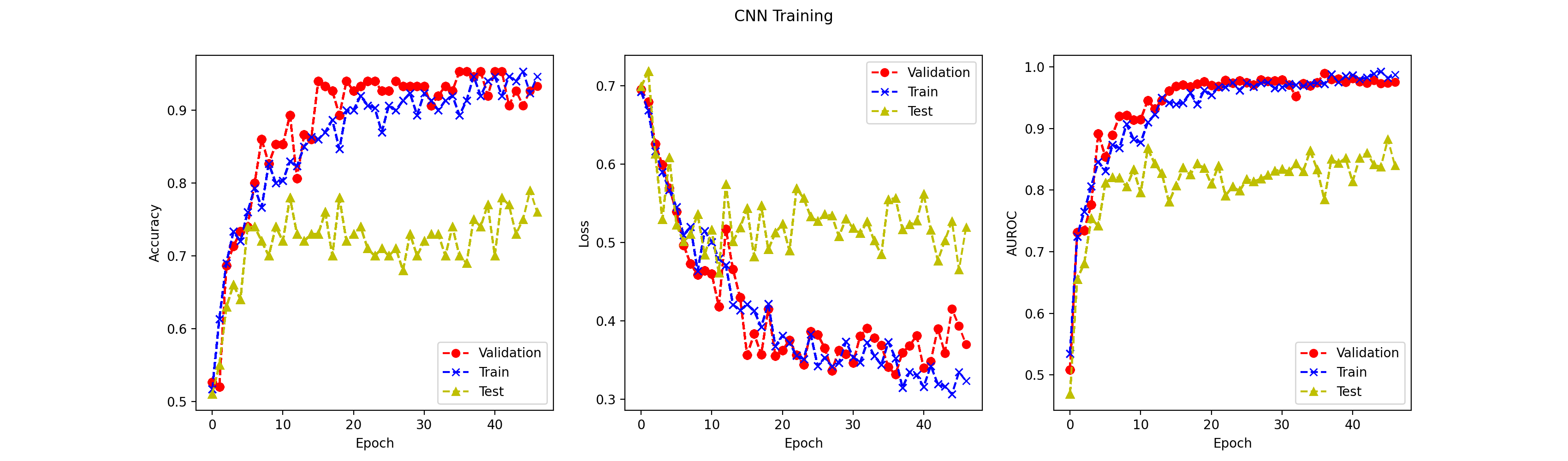
Custom challenge CNN training curve. Validation loss bottomed out at 0.3315, validation AUROC peaked at 0.9893, both at epoch 36, the checkpoint used for final predictions.
The model learned quickly through the first 10 to 20 epochs, AUROC climbing from around 0.5 toward 0.9, with training and validation curves staying close together. After epoch 20, training accuracy kept inching up while validation flattened, a normal convergence pattern rather than a sharp overfit. I selected the epoch 36 checkpoint using validation loss alone, without looking at test performance, which is the model-selection discipline that made the earlier baseline's validation-test gap so misleading in the first place.
What it's built with.
Every model, the baseline CNN, the source classifier, the transfer learning variants, the Vision Transformer, and the final custom CNN, was implemented directly in PyTorch, including the training loops, checkpointing, and early stopping logic.
What I took away.
Validation metrics can lie
The baseline CNN's 0.998 validation AUROC and 0.763 test AUROC taught me to never trust a single number. Now I always ask what the validation set actually resembles before believing what it tells me.
Freezing can be regularization
The frozen-features result was the most surprising outcome of the whole project. Less flexibility, not more, produced the best test generalization, a reminder that the model with the best validation score isn't always the model you should ship.
Architecture is only part of it
The custom CNN's biggest gains didn't come from a cleverer architecture. They came from augmentation, dropout placement, label smoothing, and honest checkpoint selection, all the unglamorous engineering around the model.
The best model didn't come from making the network as large or complex as possible. It came from understanding where the earlier models failed, controlling overfitting, and combining small architectural and training decisions into a more reliable system.